ためすう

sklearn.preprocessing.StandardScaler でデータを標準化する

2019-08-13

やったこと

sklearn.preprocessing.StandardScaler を使いデータを標準化します。

平均が0、標準偏差が1の分布に従うように調整されます。

確認環境

$ ipython --version
6.1.0
$ jupyter --version
4.3.0
$ python --version
Python 3.6.2 :: Anaconda custom (64-bit)

import sklearn
print(sklearn.__version__)

出力結果

0.21.2

調査

def printout(data):
    print("平均X: ", data[:, 0].mean())
    print("平均Y: ", data[:, 1].mean())
    print("標準偏差X: ", data[:, 0].std())
    print("標準偏差Y: ", data[:, 1].std())

from sklearn.preprocessing import StandardScaler
np.random.seed(seed=1)
data = np.random.multivariate_normal( [5, 5],  [[5, 0],[0, 2]],  10 )
print("元データ")
print(data)
printout(data)

print("---")

scaler = StandardScaler()
print("標準化")
data_std = scaler.fit_transform(data)
print(data_std)
printout(data_std)

出力結果

元データ
[[8.63214665 4.13484578]
 [3.81897206 3.48259322]
 [6.93511029 1.74513276]
 [8.90151771 3.92349088]
 [5.71339311 4.64733703]
 [8.26937274 2.08652107]
 [4.27905321 4.45686512]
 [7.53518554 3.44451885]
 [4.61443881 3.75852072]
 [5.09439281 5.82422518]]
平均X:  6.3793582926820225
平均Y:  3.7504050618892877
標準偏差X:  1.8118979237218
標準偏差Y:  1.128584883455787
---
標準化
[[ 1.24333073  0.34063962]
 [-1.41309629 -0.2372988 ]
 [ 0.30672368 -1.77680238]
 [ 1.39199863  0.15336535]
 [-0.36755116  0.79474037]
 [ 1.04311309 -1.47431001]
 [-1.15917406  0.62596981]
 [ 0.63790969 -0.27103518]
 [-0.97407225  0.007191  ]
 [-0.70918205  1.83754022]]
平均X:  -1.554312234475219e-16
平均Y:  -5.10702591327572e-16
標準偏差X:  0.9999999999999999
標準偏差Y:  1.0000000000000002

参考

sklearn.preprocessing.StandardScaler — scikit-learn 0.21.3 documentation

str.format でフォーマットする (Python)

2019-08-13

やったこと

Python の str.format を使ってみます。

確認環境

$ ipython --version
6.1.0
$ jupyter --version
4.3.0
$ python --version
Python 3.6.2 :: Anaconda custom (64-bit)

調査

print("{}-{}-{}".format("2019", "08", "12"))

出力結果

2019-08-12

参考

組み込み型 — Python 3.7.4 ドキュメント

sklearn.preprocessing.LabelEncorder を使い、カテゴリを数値化してみる

2019-08-12

やったこと

カテゴリを数値に置き換えるため、sklearn の LabelEncorder を使ってみます。

確認環境

$ ipython --version
6.1.0
$ jupyter --version
4.3.0
$ python --version
Python 3.6.2 :: Anaconda custom (64-bit)

import sklearn
print(sklearn.__version__)

出力結果

0.21.2

調査

from sklearn.preprocessing import LabelEncoder
import pandas as pd

df = pd.DataFrame([
    ['green', 'M', 10.1, 'class1'],
    ['red', 'L', 13.5, 'class2'],
    ['blue', 'XL', 15.3, 'class1']
])
df.columns = ['color', 'size', 'price', 'classlabel']
class_le = LabelEncoder()
y = class_le.fit_transform(df['classlabel'].values)
print(y)
# クラスラベルを整数から文字列に戻す
print(class_le.inverse_transform(y))

出力結果

[0 1 0]
['class1' 'class2' 'class1']

参考

sklearn.preprocessing.LabelEncoder — scikit-learn 0.21.3 documentation
Python機械学習プログラミング

numpy.sort、numpy.argsort を使う

2019-08-12

やったこと

numpy.sort、numpy.argsort を使い、配列をソートします。

確認環境

$ ipython --version
6.1.0
$ jupyter --version
4.3.0
$ python --version
Python 3.6.2 :: Anaconda custom (64-bit)

import numpy as np
np.__version__

出力結果

'1.16.4'

調査

numpy.sort

a = np.array([[1,4, 0],[3,1, -2]])
print(np.sort(a))

出力結果

[[ 0  1  4]
 [-2  1  3]]

numpy.argsort

a = np.array([[1,4, 0],[3,1, -2]])
print(np.argsort(a))

出力結果

[[2 0 1]
 [2 1 0]]

np.argsort ではインデックスが返却されることが確認できました。

参考

欠損値を補完する (scikit-learn SimpleImputer)

2019-08-12

やったこと

pandas の isnull を使い欠測値をカウントします。

確認環境

$ ipython --version
6.1.0
$ jupyter --version
4.3.0
$ python --version
Python 3.6.2 :: Anaconda custom (64-bit)

import sklearn
print(sklearn.__version__)

出力結果

0.21.2

調査

Imputer (Deprecated)

import pandas as pd
from sklearn.preprocessing import Imputer
df = pd.DataFrame({'A':[1,2,3,4,5], 'B':[1,2,None,None,5], 'C':[None, None, 3, None, 4]})

imr = Imputer(missing_values='NaN', strategy='mean', axis=0)
imr = imr.fit(df)
imr.transform(df.values)

出力結果

/anaconda3/lib/python3.6/site-packages/sklearn/utils/deprecation.py:66: DeprecationWarning: Class Imputer is deprecated; Imputer was deprecated in version 0.20 and will be removed in 0.22. Import impute.SimpleImputer from sklearn instead.
  warnings.warn(msg, category=DeprecationWarning)

array([[1.        , 1.        , 3.5       ],
       [2.        , 2.        , 3.5       ],
       [3.        , 2.66666667, 3.        ],
       [4.        , 2.66666667, 3.5       ],
       [5.        , 5.        , 4.        ]])

SimpleImputer

import pandas as pd
from sklearn.impute import SimpleImputer

df = pd.DataFrame({'A':[1,2,3,4,5], 'B':[1,2,None,None,5], 'C':[None, None, 3, None, 4]})
imr = SimpleImputer( strategy='mean')
imr.fit(df)
imr.transform(df.values)

出力結果

array([[1.        , 1.        , 3.5       ],
       [2.        , 2.        , 3.5       ],
       [3.        , 2.66666667, 3.        ],
       [4.        , 2.66666667, 3.5       ],
       [5.        , 5.        , 4.        ]])

参考

sklearn.preprocessing.Imputer — scikit-learn 0.21.3 documentation

numpy.var を使って分散を求める

2019-08-12

やったこと

numpy.var を使い分散を求めます。

確認環境

$ ipython --version
6.1.0
$ jupyter --version
4.3.0
$ python --version
Python 3.6.2 :: Anaconda custom (64-bit)

import numpy as np
np.__version__

出力結果

'1.16.4'

調査

import numpy as np
a = np.array([[10, 20], [60, 80]])
mean = np.mean(a)
print("平均: ", mean)
print("分散: ", np.var(a))
print('--- 手動計算 ---')
var_result = sum([(x-mean)**2 for x in a.ravel()]) / len(a.ravel())
print("分散: ", var_result)

出力結果

平均:  42.5
分散:  818.75
--- 手動計算 ---
分散:  818.75

参考

numpy.var — NumPy v1.17 Manual

numpy.reshape を使ってみる

2019-08-12

やったこと

配列を新しい形に変えるため、numpy.reshape を使ってみます。

確認環境

$ ipython --version
6.1.0
$ jupyter --version
4.3.0
$ python --version
Python 3.6.2 :: Anaconda custom (64-bit)

import numpy as np
np.__version__

出力結果

'1.16.4'

調査

import numpy as np
a = np.arange(10, 22)
print(a)
print(a.reshape((4, 3)))

出力結果

[10 11 12 13 14 15 16 17 18 19 20 21]
[[10 11 12]
 [13 14 15]
 [16 17 18]
 [19 20 21]]

参考

numpy.reshape — NumPy v1.17 Manual

pandas.DataFrame.dropna で欠損値を削除する

2019-08-11

やったこと

pandas の droopna を使い欠測値をカウントします。

確認環境

$ ipython --version
6.1.0
$ jupyter --version
4.3.0
$ python --version
Python 3.6.2 :: Anaconda custom (64-bit)

pd.__version__

出力結果

'0.20.3'

調査

import pandas as pd
df = pd.DataFrame({'A':[1,2,3,4,5], 'B':[1,2,None,None,5], 'C':[None, None, 3, None, 4]})
print(df.dropna())
print('---')
print(df.dropna(axis=1))

出力結果

   A    B    C
4  5  5.0  4.0
---
   A
0  1
1  2
2  3
3  4
4  5

参考

pandas.DataFrame.dropna — pandas 0.25.0 documentation

pandas.DataFrame.isnull で欠損値をカウントする

2019-08-11

やったこと

pandas の isnull を使い欠測値をカウントします。

確認環境

$ ipython --version
6.1.0
$ jupyter --version
4.3.0
$ python --version
Python 3.6.2 :: Anaconda custom (64-bit)

pd.__version__

'0.20.3'

調査

import pandas as pd
df = pd.DataFrame({'A':[1,2,3,4,5], 'B':[1,2,None,None,5], 'C':[None, None, 3, None, 4]})
print(df.isnull().sum())
print('---')
print(df.isnull().sum(axis=1))

出力結果

A    0
B    2
C    3
dtype: int64
0    1
1    1
2    1
3    2
4    0
dtype: int64

参考

pandas.DataFrame.isnull — pandas 0.25.0 documentation

Matplotlib を使ってみる

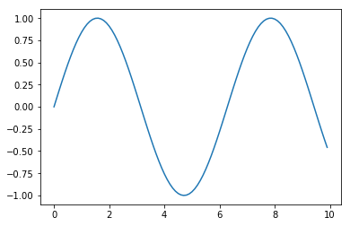
2019-08-10

やったこと

Matplotlib を使って、グラフを描画してみます。

確認環境

$ ipython --version
6.1.0
$ jupyter --version
4.3.0
$ python --version
Python 3.6.2 :: Anaconda custom (64-bit)

調査

import matplotlib.pyplot as plt
%matplotlib inline

x = np.arange(0, 10, 0.1)
y = np.sin(x)
plt.plot(x, y)

%matplotlib inline は、Jupyter Notebook でグラフを表示するようにします。

画像

参考

matplotlib.pyplot — Matplotlib 3.1.0 documentation