ためすう
Ruby で casecmp を使ってみる
2019-09-02やったこと
Ruby で casecmp を使ってみます。
確認環境
$ ruby --version
ruby 2.6.3p62 (2019-04-16 revision 67580) [x86_64-darwin17]
調査
$ irb
...
irb(main):007:0> words = ['abc', 'Abc', 'ABC', 'aaa']
=> ["abc", "Abc", "ABC", "aaa"]
irb(main):008:0> words.each do |r|
irb(main):009:1*   p r.casecmp('abc')
irb(main):010:1>   p 'abc'.casecmp(r)
irb(main):011:1>   p 'end!!!'
irb(main):012:1> end
0
0
"end!!!"
0
0
"end!!!"
0
0
"end!!!"
-1
1
"end!!!"
=> ["abc", "Abc", "ABC", "aaa"]
参考
OpenAPI Generator を使ってみる
2019-08-27やったこと
OpenAPI Generator を使ってみます
スタブサーバーを作成する
$ GENERATOR=spring
$ docker run --rm -v ${PWD}:/local \
  openapitools/openapi-generator-cli generate \
  -i /local/openapi.yaml \
  -g ${GENERATOR} \
  -o /local/out/${GENERATOR} \
  --additional-properties returnSuccessCode=true
$ docker run --rm -v ${PWD}:/usr/src/mymaven \
-w /usr/src/mymaven maven mvn package$ docker run --rm -p 3000:3000 \
-v ${PWD}:/usr/src/myapp -w /usr/src/myapp \
java java -jar target/openapi-spring-1.0.0.jarhttp://localhost:3000/posts にアクセスして、モックのデータを取得することができました。
その他
- python-flask
- ruby-on-rails
flask や rails もあったのですが、都度実装が必要そうでした。
参考
- WEB+DB vol.108
Swagger UI を使ってみる
2019-08-26やったこと
Swagger UI を使ってみます
調査
Swagger UI を表示する環境を準備
$ docker pull swaggerapi/swagger-ui
$ docker run -p 80:8080 swaggerapi/swagger-ui
http://localhost:8080/ で Swagger UI が利用できるようになります。
Swagger UI から Web API サーバーへアクセスできるようにする
Gemfile
gem 'rack-cors', :group => :development$ bundle installconfig/initializers/cors.rb
Rails.application.config.middleware.insert_before 0, Rack::Cors do
  allow do
    origins '*'
    resource '*', headers: :any, methods: [:get, :post, :options]
  end
end
openapi.yml はこの記事で書いたものを利用します。
※ public ディレクトリに配置しました。
http://localhost:3000/openapi.yml で Exploreすると利用できます。
課題
実運用するときには、外から見えない位置に openapi.yml を配置する必要があると思いました。
参考
Swagger Editor を使ってみる
2019-08-25やったこと
Swagger Editor を使ってみます
調査
Swagger Editor を github から clone する
$ git clone https://github.com/swagger-api/swagger-editor.gitローカルで Swagger Editor を起動する
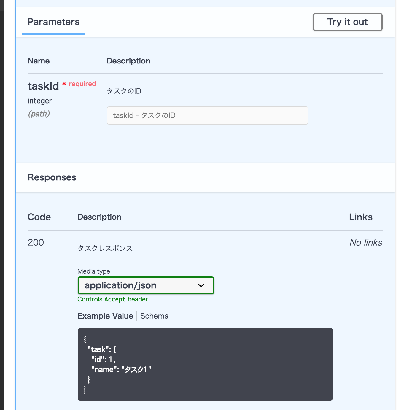
$ open swagger-editor/index.htmlSwagger Editor を書いてみる
例は下記です。
# swaggerのバージョン定義
openapi: "3.0.2"
info:
  title: "タスク情報API"
  version: "1.0.0"
  description: "desc...."
servers:
  - url: http://localhost:3000
    description: Local server
paths:
  /tasks/show:
    get:
      description: タスク詳細を取得する
      operationId: getTask
      parameters:
        - $ref: '#/components/parameters/taskIdParam'
      responses:
        '200':
          $ref: '#/components/responses/Task'
components:
  schemas:
    Task:
      type: object
      properties:
        task:
          $ref: '#/components/schemas/TaskProperties'
    TaskProperties:
      type: object
      properties:
        id:
          type: integer
          example: 1
        name:
          type: string
          example: 'タスク1'
  parameters:
    taskIdParam:
      name: taskId
      in: path
      description: タスクのID
      required: true
      schema:
        type: integer
  responses:
    Task:
      description: タスクレスポンス
      content:
        application/json:
          schema:
            $ref: '#/components/schemas/Task'
イメージ
参考
Rails で autodoc を使ってみる
2019-08-25やったこと
Rails で API ドキュメントを生成する autodoc を使ってみます。
確認環境
$ ruby --version
ruby 2.6.3p62 (2019-04-16 revision 67580) [x86_64-darwin17]

$ rails --version
Rails 5.2.3
調査
Gemfile
group :development, :test do
  # ... something
  gem 'autodoc'
end
$ bundle installapp/controllers/tasks_controller.rb
class TasksController < ApplicationController
  def show
    point = Struct.new(:x, :y)
    tmp = point.new(111, 222)

    render :json => tmp.to_json
  end
end
rspec の実行 + APIのドキュメント生成
spec/requests/task_apis_spec.rb
require 'rails_helper'
RSpec.describe "TaskApis", type: :request do
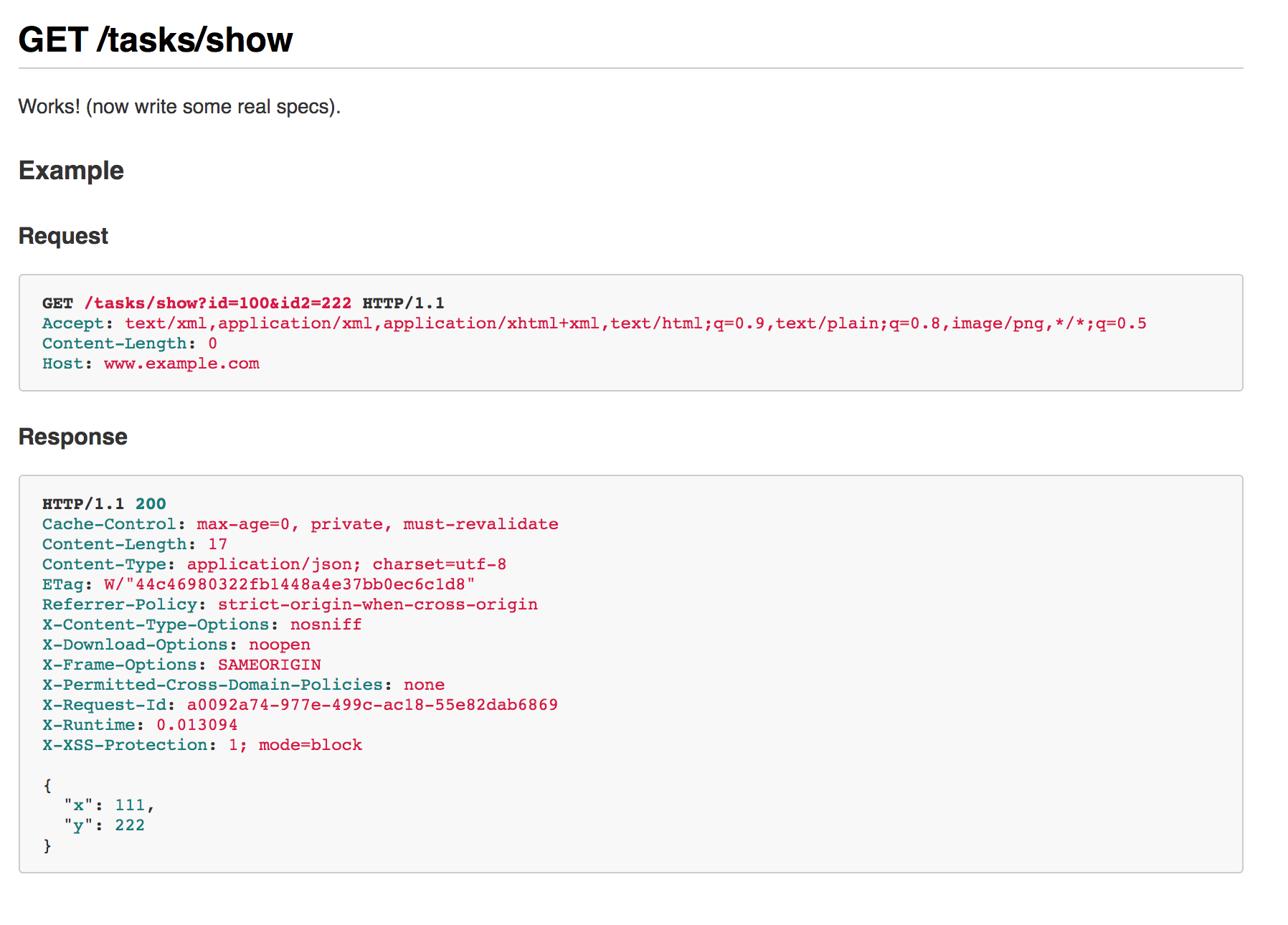
describe "GET /tasks/show" do
it "works! (now write some real specs)", :autodoc do
parameters = {id: 100, id2: 222}
get '/tasks/show', params: parameters
expect(response).to have_http_status(200)
end
end
end$ AUTODOC=1 bundle exec rspec spec/requests/task_apis_spec.rb出力結果
doc/task_apis.md に出力されます。
今回は、内容をキャプチャに記載します。
参考
Python の zip 関数を使ってみる
2019-08-23やったこと
Python の zip 関数を使ってみます。
確認環境
$ python
Python 3.6.2 |Anaconda custom (64-bit)| (default, Sep 21 2017, 18:29:43)
[GCC 4.2.1 Compatible Clang 4.0.1 (tags/RELEASE_401/final)] on darwin
Type "help", "copyright", "credits" or "license" for more information.
調査
>>> x = [1, 2, 3]
>>> y = [4, 5, 6]
>>> zip(x, y)
<zip object at 0x10ef954c8>
>>> for a, b in zip(x, y):
...   print(a, b)
...
1 4
2 5
3 6
参考
matplotlib.pyplot.barh を使って、棒グラフを表示する
2019-08-15やったこと
matplotlib.pyplot.barh を使ってみます
確認環境
$ ipython --version
6.1.0
$ jupyter --version
4.3.0
$ python --version
Python 3.6.2 :: Anaconda custom (64-bit)
import matplotlib
matplotlib.__version__出力結果
'2.0.2'調査
import matplotlib.pyplot as plt
%matplotlib inline

y = [10, 20, 30]
x = [60, 50, 80]
plt.barh(y, x, height=5)
出力結果
<Container object of 3 artists>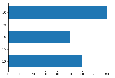
参考
matplotlib.pyplot.subplot を使ってみる
2019-08-15やったこと
matplotlib.pyplot.subplot を使ってみます
確認環境
$ ipython --version
6.1.0
$ jupyter --version
4.3.0
$ python --version
Python 3.6.2 :: Anaconda custom (64-bit)
import matplotlib
matplotlib.__version__出力結果
'2.0.2'調査
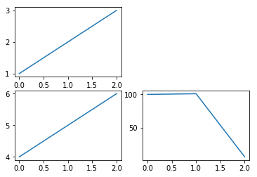
import matplotlib.pyplot as plt
%matplotlib inline

plt.subplot(221)
plt.plot([1,2,3])


plt.subplot(223)
plt.plot([4, 5, 6])

plt.subplot(224)
plt.plot([100, 101, 6])
出力結果
参考
やったこと
sklearn.ensemble.RandomForestClassifier を利用して、
RandomForest 学習させてみます。
確認環境
$ ipython --version
6.1.0
$ jupyter --version
4.3.0
$ python --version
Python 3.6.2 :: Anaconda custom (64-bit)
import sklearn
print(sklearn.__version__)出力結果
0.21.2調査
特徴のラベル
1) Alcohol
2) Malic acid
3) Ash
4) Alcalinity of ash
5) Magnesium
6) Total phenols
7) Flavanoids
8) Nonflavanoid phenols
9) Proanthocyanins
10)Color intensity
11)Hue
12)OD280/OD315 of diluted wines
13)Proline
RandoForest で学習してみる
import pandas as pd
df_wine = pd.read_csv('https://archive.ics.uci.edu/ml/machine-learning-databases/wine/wine.data', header=None)

from sklearn.ensemble import RandomForestClassifier
X, y = df_wine.iloc[:, 1:].values, df_wine.iloc[:, 0].values

from sklearn.model_selection import train_test_split
X_train, X_test, y_train, y_test = train_test_split(X, y, test_size=0.3, random_state=0)

forest = RandomForestClassifier(n_estimators=10000, random_state=0, n_jobs=-1)
forest.fit(X_train, y_train)

# 特徴の重要度を取得
importances = forest.feature_importances_
結果を表示する
indicies = np.argsort(importances)[::-1]
for f in range(X_train.shape[1]):
    print("%2d) label: %s importance: %f" % (f + 1, indicies[f], importances[indicies[f]]))
出力結果
 1) label: 9 importance: 0.182483
 2) label: 12 importance: 0.158610
 3) label: 6 importance: 0.150948
 4) label: 11 importance: 0.131987
 5) label: 0 importance: 0.106589
 6) label: 10 importance: 0.078243
 7) label: 5 importance: 0.060718
 8) label: 3 importance: 0.032033
 9) label: 1 importance: 0.025400
10) label: 8 importance: 0.022351
11) label: 4 importance: 0.022078
12) label: 7 importance: 0.014645
13) label: 2 importance: 0.013916
参考
やったこと
sklearn.preprocessing.MinMaxScaler を使いデータを正規化します。
データを 0~1 の範囲にスケーリングし直します。
確認環境
$ ipython --version
6.1.0
$ jupyter --version
4.3.0
$ python --version
Python 3.6.2 :: Anaconda custom (64-bit)
import sklearn
print(sklearn.__version__)出力結果
0.21.2調査
def printout(data):
    print("平均X: ", data[:, 0].mean())
    print("平均Y: ", data[:, 1].mean())
    print("標準偏差X: ", data[:, 0].std())
    print("標準偏差Y: ", data[:, 1].std())
    print("MIN X: ", data[:, 0].min())
    print("MIN Y: ", data[:, 1].min())
    print("MAX X: ", data[:, 0].max())
    print("MAX Y: ", data[:, 1].max())

from sklearn.preprocessing import MinMaxScaler
np.random.seed(seed=1)
data = np.random.multivariate_normal( [5, 5],  [[5, 0],[0, 2]],  10 )
print("元データ")
print(data)
printout(data)

print("---")

scaler = MinMaxScaler()
print("正規化")
data_norm = scaler.fit_transform(data)
print(data_norm)
printout(data_norm)
出力結果
元データ
[[8.63214665 4.13484578]
 [3.81897206 3.48259322]
 [6.93511029 1.74513276]
 [8.90151771 3.92349088]
 [5.71339311 4.64733703]
 [8.26937274 2.08652107]
 [4.27905321 4.45686512]
 [7.53518554 3.44451885]
 [4.61443881 3.75852072]
 [5.09439281 5.82422518]]
平均X:  6.3793582926820225
平均Y:  3.7504050618892877
標準偏差X:  1.8118979237218
標準偏差Y:  1.128584883455787
MIN X:  3.8189720581437347
MIN Y:  1.7451327605454043
MAX X:  8.901517712729385
MAX Y:  5.82422517959429
---
正規化
[[0.94700076 0.58584429]
 [0.         0.4259429 ]
 [0.6131058  0.        ]
 [1.         0.5340301 ]
 [0.37273075 0.71148284]
 [0.87562434 0.08369222]
 [0.0905218  0.66478816]
 [0.73117169 0.41660887]
 [0.15650951 0.49358724]
 [0.25094133 1.        ]]
平均X:  0.5037605972566557
平均Y:  0.4915976632398656
標準偏差X:  0.35649417572610337
標準偏差Y:  0.2766754874651595
MIN X:  0.0
MIN Y:  0.0
MAX X:  1.0
MAX Y:  1.0